Tick Size and Discrete Control in Prediction Markets

Prediction-market prices lie in a bounded interval,

$$p \in [0,1],$$

with integer inventory and discrete tick size $\Delta$.

For markets such as Kalshi, $\Delta$ is commonly $0.01$ and can be as small as $0.001$. Since the full price range has width $1$, the exchange grid is not always negligible relative to the price adjustments produced by a continuous market-making model.

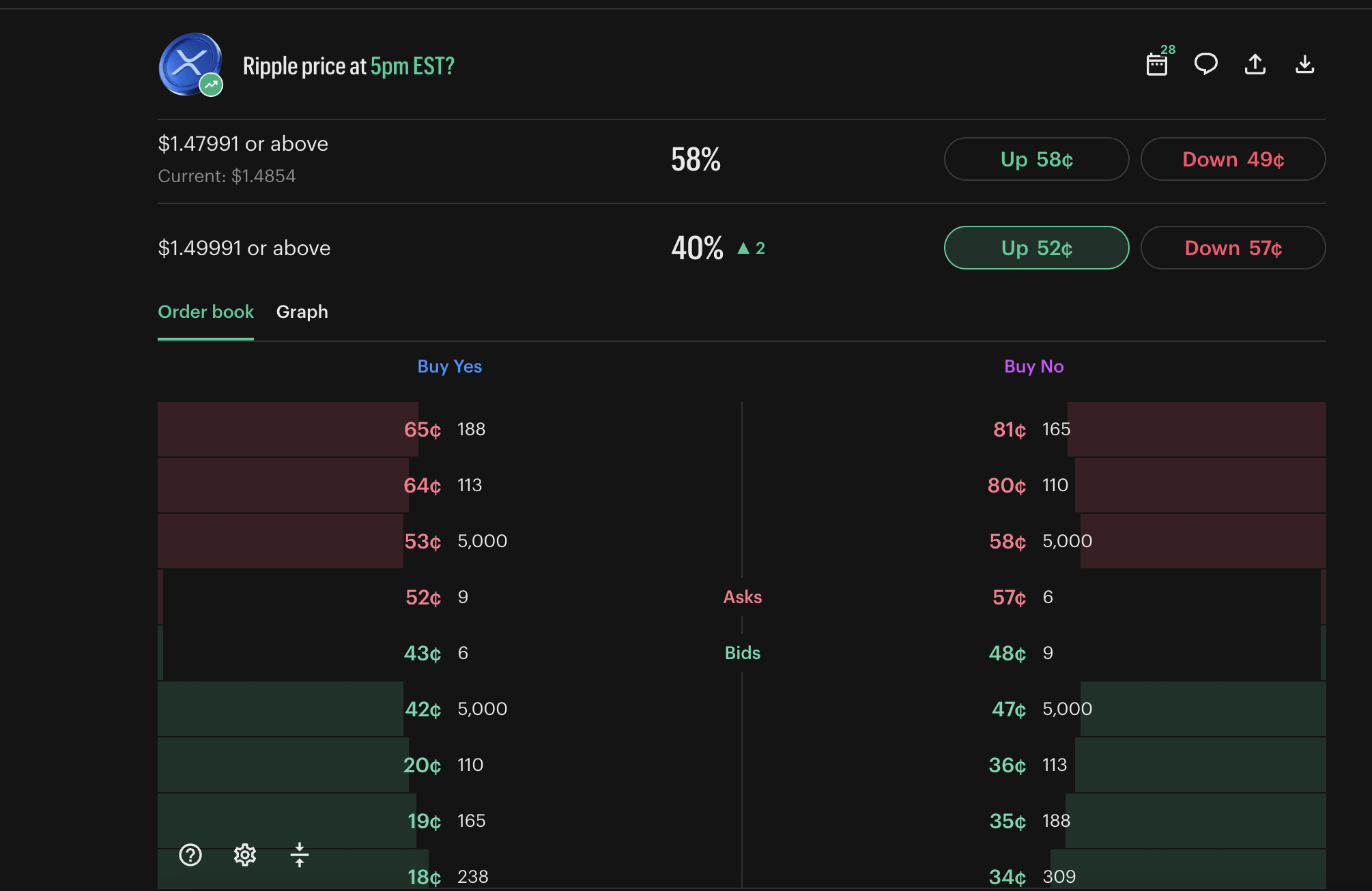
A live prediction-market order book. Every resting quote sits on a discrete cent grid, so the executable prices are exactly the admissible set $\mathcal P_\Delta$ we work with below.

Start with the Avellaneda-Stoikov reservation price

$$r(q,t) = S_t-q\gamma\sigma^2(T-t),$$

where $q\in\mathbb Z$ is inventory. Define

$$\nu_t = \gamma\sigma^2(T-t).$$

Then

$$r(q+1,t)-r(q,t) = -\nu_t.$$

Thus $\nu_t$ is the change in reservation price induced by one unit of inventory.

On the exchange, admissible prices are

$$\mathcal P_\Delta = \{0,\Delta,2\Delta,\ldots,1\}.$$

Define nearest-tick quantization

$$Q_\Delta(x) = \Delta \operatorname{round} \left( \frac{x}{\Delta} \right),$$

and the executable reservation price

$$\widehat r(q,t) = \Pi_{[0,1]} \left( Q_\Delta(r(q,t)) \right),$$

where $\Pi_{[0,1]}$ clips the price to the prediction-market domain.

Away from the boundaries,

$$|Q_\Delta(r)-r| \leq \frac{\Delta}{2}.$$

The relevant dimensionless ratio is

$$\boxed{ \rho_t = \frac{\Delta}{\nu_t} = \frac{\Delta} {\gamma\sigma^2(T-t)}. }$$

If

$$\rho_t \ll 1,$$

then one inventory change moves the reservation price through several ticks.

If

$$\rho_t \approx 1,$$

then one inventory change moves the reservation price by roughly one tick.

If

$$\rho_t \gg 1,$$

then several inventory changes can occur before the executable reservation price changes.

For example, let

$$S_t=0.50, \qquad \nu_t=0.002, \qquad \Delta=0.01.$$

Then

$$\rho_t = \frac{0.01}{0.002} = 5.$$

The continuous reservation prices are

$$0.500,\; 0.498,\; 0.496,\; 0.494,\; 0.492,\; 0.490,\ldots$$

while the exchange only admits

$$0.50,\; 0.49,\; 0.48,\ldots$$

After quantization, several distinct inventory states can therefore map to the same price.

For $\nu_t<\Delta$,

$$\widehat r(q+1,t)-\widehat r(q,t) \in \{0,-\Delta\},$$

away from the $0$ and $1$ boundaries.

The continuous model instead gives

$$r(q+1,t)-r(q,t) = -\nu_t.$$

Tick transitions occur when

$$S_t-q\nu_t = \left(k+\frac12\right)\Delta.$$

Solving for the corresponding inventory levels,

$$q_k = \frac{ S_t-(k+\frac12)\Delta }{ \nu_t }.$$

Therefore consecutive transitions satisfy

$$|q_{k+1}-q_k| = \frac{\Delta}{\nu_t} = \rho_t.$$

Hence

$$\boxed{ \rho_t = \text{inventory spacing between consecutive tick transitions}. }$$

For $\rho_t=5$, consecutive price changes are separated by approximately five units of inventory.

The bounded price interval adds another discretization effect. If

$$r(q,t)\leq0,$$

then

$$\widehat r(q,t)=0,$$

and if

$$r(q,t)\geq1,$$

then

$$\widehat r(q,t)=1.$$

Thus the executable policy is piecewise constant both because of tick quantization inside $(0,1)$ and because of saturation at the boundaries.

The same issue appears in quote optimization.

Suppose the continuous model produces a local objective $H(p)$. The continuous problem is

$$p^* = \arg\max_{p\in[0,1]} H(p).$$

The exchange problem is

$$\boxed{ p_\Delta^* = \arg\max_{p\in\mathcal P_\Delta}H(p). }$$

For $\Delta=0.01$,

$$|\mathcal P_\Delta|=101,$$

while for $\Delta=0.001$,

$$|\mathcal P_\Delta|=1001.$$

If $H$ is twice differentiable near an interior maximizer $p^*$ and

$$|H''(p)|\leq M,$$

then the nearest admissible grid point $\widehat p_\Delta$ satisfies

$$|\widehat p_\Delta-p^*| \leq \frac{\Delta}{2}.$$

Since

$$H'(p^*)=0,$$

Taylor expansion gives

$$H(p^*)-H(\widehat p_\Delta) \leq \frac{M\Delta^2}{8}.$$

Because $p_\Delta^*$ is the optimal point on the grid,

$$0 \leq H(p^*)-H(p_\Delta^*) \leq \frac{M\Delta^2}{8}.$$

Therefore

$$H(p_\Delta^*) \to H(p^*)$$

as

$$\Delta\to0.$$

The continuous optimization is recovered as the fine-grid limit of the discrete problem.

For the inventory adjustment, this limit corresponds to

$$\frac{\Delta} {\gamma\sigma^2(T-t)} \to0.$$

At finite tick size, the natural control problem instead has discrete prices and integer inventory. With state

$$s=(p,q),$$

and actions

$$a\in\mathcal P_\Delta,$$

the value function can be written in Bellman form as

$$V(s) = \max_{a\in\mathcal A(s)} \left[ R(s,a) + \beta \sum_{s'} P(s'|s,a)V(s') \right].$$

This gives the relation

$$\boxed{ \text{discrete prediction-market control} \;\xrightarrow{\Delta\to0}\; \text{continuous market-making control}. }$$

For finite $\Delta$, the key scale is

$$\boxed{ \rho_t = \frac{\Delta} {\gamma\sigma^2(T-t)}. }$$

When $\rho_t\ll1$, the discrete grid approximates the continuous inventory adjustment.

When $\rho_t\gtrsim1$, multiple inventory states map to the same admissible price and the discrete control problem differs locally from its continuous approximation.