The Geometry of Position in a Transformer

RoPE gives transformers an explicit geometric representation of relative position inside attention. Each two-dimensional query/key plane rotates with a fixed frequency $\left(\frac{\theta}{\text{token}}\right)$,

$$R_k(t)= \begin{bmatrix} \cos(\omega_k t) & -\sin(\omega_k t)\\ \sin(\omega_k t) & \cos(\omega_k t) \end{bmatrix}$$

But RoPE is applied to queries and keys, not written directly into the residual stream. After attention, value mixing, residual additions, and MLPs, what notion of position remains, and how does it evolve as it passes through the layers of the transformer?

We studied exactly this in Qwen2.5-3B. The code is on GitHub.

For a given phrase $x$, layer $\ell$, base position $b=10$, and displacement $\Delta$, define

$$p_{\ell,x}(\Delta) = h_{\ell}(x, b+\Delta) - h_{\ell}(x, b),$$

and average over a set of phrases,

$$p_{\ell}(\Delta) = \mathbb{E}[p_{\ell,x}(\Delta)].$$

We use 20 short matched phrases and move them over

$$\Delta \in \{100, 102, \dots, 600\}.$$

To avoid confounds from the additional context, filler tokens between the two locations are masked from the moved phrase's attention. The phrase nevertheless remains at its true later token index, so RoPE is still evaluated at $b+\Delta$. The resulting map

$$(\ell, \Delta) \mapsto p_{\ell}(\Delta)$$

gives an empirical geometry of implicit position inside the residual stream.

Displacing Tokens by Δ

For fixed $\Delta$, positional displacement is highly consistent across phrase content through much of the model. Under the matched-context intervention, pairwise cosine similarity between displacement vectors from different phrases is often above $0.99$. Thus, to first order,

$$p_{\ell,x}(\Delta) \approx p_{\ell}(\Delta) + \epsilon_{\ell,x}(\Delta).$$

From this, we vary $\Delta$ to see what structure, if any, emerges. We chose an arbitrary middle layer, layer 15, and computed the cosine Gram matrix

$$C_{\ell}(i,j) = \frac{p_{\ell}(\Delta_i)^\top p_{\ell}(\Delta_j)}{\|p_{\ell}(\Delta_i)\|\,\|p_{\ell}(\Delta_j)\|},$$

which shows repeated blocks and cross-like patterns across multiple positional scales.

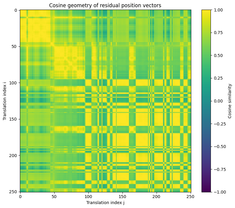
The layer-15 cosine Gram matrix over displacements: clearly non-random, with repeated blocks and cross-like structure across multiple positional scales.

This geometry is clearly not random and very visibly multiscale.

Qwen's Inherent Frequencies

Qwen2.5-3B uses 64 RoPE frequencies,

$$\omega_k = \theta^{-2k/128},\quad \theta=10^6,\quad k \in \{0, \dots, 63\}.$$

Therefore a natural coordinate system for describing a displacement by $\Delta$ is

$$d_{\text{RoPE}}(\Delta) = \begin{bmatrix} \cos(\omega_1\Delta)-1\\ \sin(\omega_1\Delta)\\ \vdots\\ \cos(\omega_{64}\Delta)-1\\ \sin(\omega_{64}\Delta) \end{bmatrix} \in \mathbb{R}^{128}.$$

We ask whether the residual position vector is approximately a linear image of this known architectural trajectory:

$$p_{15}(\Delta) \approx B^\top d_{\text{RoPE}}(\Delta).$$

Over a ~500 token window, the 128 RoPE features are not all distinguishable. For small $\omega$,

$$\sin(\omega\Delta) \approx \omega\Delta, \qquad \cos(\omega\Delta) - 1 \approx -\tfrac{1}{2}\omega^2\Delta^2,$$

so many low-frequency coordinates become numerically redundant. The singular spectrum of the RoPE design matrix has a sharp cutoff at approximately $r = 42$.

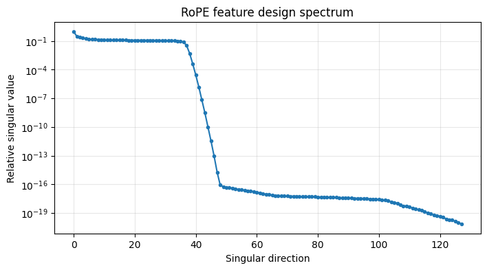
Singular spectrum of the RoPE design matrix over the finite window. It falls off a cliff after roughly 42 directions: low frequencies collapse into numerical redundancy, leaving $r \approx 42$ usable coordinates.

Using only these 42 numerically supported directions, fitting $B$ on 80% of the sampled displacements and evaluating on held-out $\Delta$ gives

$$\boxed{ \text{mean vector cosine} = 0.912 } \qquad \boxed{ \text{Gram cosine} = 0.941 }$$

The corresponding relative errors are $0.392$ for the vectors and $0.338$ for the Gram matrix. Therefore the model captures the geometry much better than the exact amplitudes.

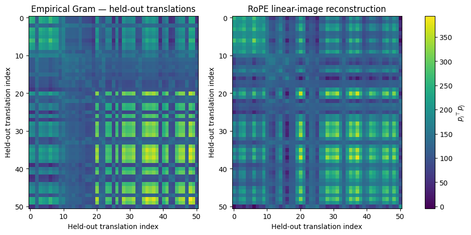
Held-out displacements: the empirical Gram matrix (left) versus its reconstruction from a linear image of Qwen's RoPE coordinates (right). The geometry is recovered well even where the exact amplitudes are not.

This is stronger than simply observing similar Fourier peaks: much of the held-out residual positional trajectory can be reconstructed from a linear mixture of Qwen's actual RoPE coordinates.

The frequency specificity is real but modest. Across 20 controls formed by perturbing each Qwen frequency multiplicatively in log-space, the mean held-out vector cosine was $0.895$, with a maximum of $0.907$, compared with $0.912$ for the exact Qwen ladder. Thus the result is best stated as:

Residual position is strongly Fourier/RoPE-like, with additional specificity to Qwen's exact frequencies.

A nearby Fourier basis can explain much of the same finite-window trajectory.

What About Depth?

For each layer, collect all positional vectors into

$$P_\ell = \begin{bmatrix} p_\ell(\Delta_1)^\top\\ \vdots\\ p_\ell(\Delta_{251})^\top \end{bmatrix} \in \mathbb{R}^{251\times2048}.$$

The cosine geometry of $P_\ell$ changes sharply in the first few layers, then becomes remarkably stable through most of the network.

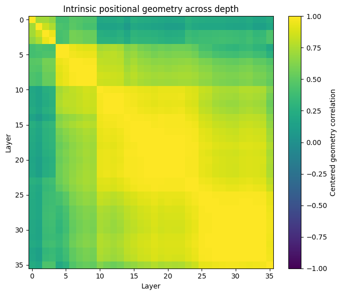
Centered geometry correlation between layers. After the first few layers the intrinsic positional geometry is remarkably stable (the large bright block).

At the same time, the vectors themselves do not remain fixed in residual coordinates. Their orientation steadily changes with depth, while their norms grow substantially toward the final layers.

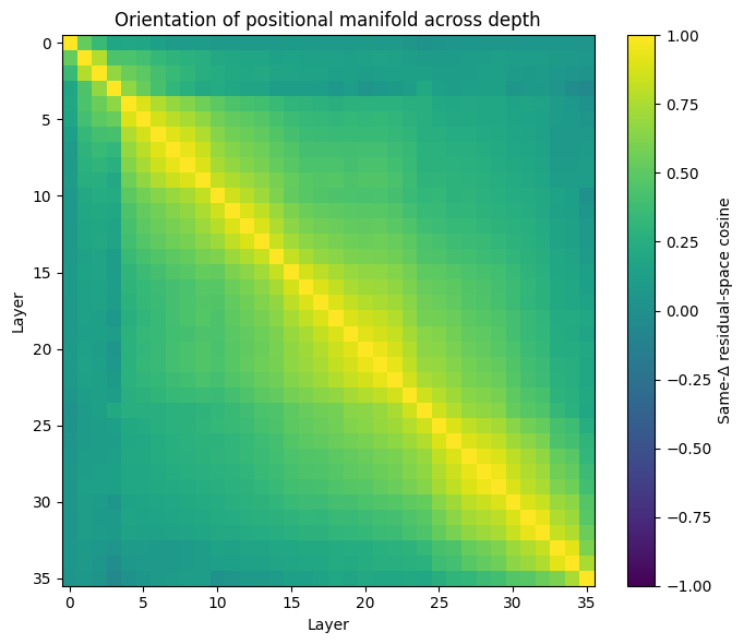
Same-$\Delta$ residual-space cosine between layers. The bright diagonal band shows the manifold's orientation drifting steadily with depth rather than staying fixed.

This suggests that the positional manifold is being transported through residual space. A first model is scaled orthogonal transport,

$$P_{\ell+1} \approx s_\ell P_\ell R_\ell, \qquad R_\ell^\top R_\ell = I.$$

This works surprisingly well for most adjacent layers, but it is not sufficient. A general linear map performs substantially better:

$$\boxed{ P_{\ell+1} \approx P_\ell M_\ell. }$$

To test this without interpolating the sampled positions, we construct a rank-42 shared basis using only training values of $\Delta$, fit $M_\ell$ on 80% of displacements, and evaluate on the remaining 20%. For most middle layers, held-out error inside this subspace is only 0.4% to 1.5%. When mapped back into the full 2048-dimensional residual space, errors are about 3% to 4%.

Most of this full-space error is simply the rank-42 projection floor. For example,

$$20\to21: \qquad \text{reduced} = 0.0040, \quad \text{full} = 0.0343, \quad \text{projection} = 0.0341,$$

and likewise

$$28\to29: \qquad 0.0038,\quad 0.0281,\quad 0.0279.$$

The linear map accounts for almost all predictable evolution of the resolved positional manifold. There are, however, several genuine reorganization points. The strongest is $3\to4$, where full-space prediction error rises to approximately $0.119$ despite a projection error of only $0.018$.

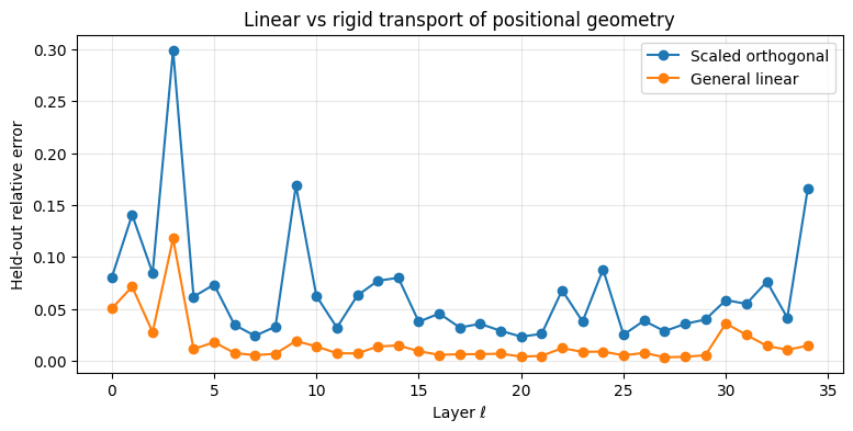
Held-out transport error per layer: a general linear map (orange) tracks the manifold's evolution far better than scaled-orthogonal transport (blue), and the 3→4 spike marks a genuine reorganization.

The dominant depth dynamics are therefore not only rotation and uniform scaling. Writing the polar decomposition

$$M_\ell = R_\ell S_\ell,$$

the orthogonal factor $R_\ell$ changes orientation, while the positive-semidefinite factor $S_\ell$ selectively stretches and contracts positional directions. The implicit representation of position is approximately linearly transported, but anisotropically.

Conclusion

Across token displacement,

$$\Delta \mapsto p_\ell(\Delta),$$

the residual stream contains a multiscale positional manifold strongly related to the model's RoPE coordinates:

$$p_\ell(\Delta) \approx B_\ell\, d_{\text{RoPE}}(\Delta).$$

Across network depth,

$$\ell \mapsto p_\ell(\Delta),$$

that manifold is transformed approximately linearly:

$$p_{\ell+1}(\Delta) \approx M_\ell\, p_\ell(\Delta).$$

So an implicit position vector is neither a fixed vector added to the residual stream nor simply the original RoPE rotation copied downstream. Instead, position appears as a structured low-dimensional manifold whose oscillatory geometry is inherited from RoPE and whose embedding is progressively rotated, stretched, and occasionally reorganized as computation moves through the transformer. The object is naturally

$$\boxed{ (\ell,\Delta) \longmapsto p_\ell(\Delta). }$$

RoPE determines much of its geometry along $\Delta$; the transformer supplies an approximately linear evolution along $\ell$.