Partition Geometry: Profile Complexity and the Axis-Alignment Tax
Decision trees, ReLU networks, and linear models all do the same thing at heart: they partition space into regions and assign a label to each. They just do it with different primitives. A tree stacks axis-aligned cuts; a linear model draws one oblique hyperplane; a ReLU network folds space with layered hyperplanes. Partition geometry is a small framework for comparing these mechanisms on equal footing, by laying them on the same labeled grid and asking how expensive the target is for each.
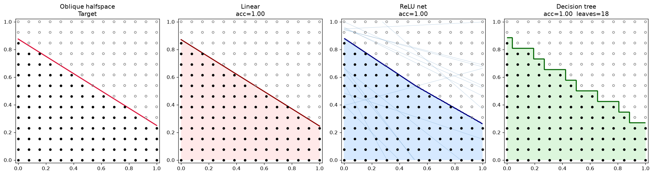
The same oblique-halfspace target under three mechanisms. A linear model needs one cut, a ReLU net folds space with many hyperplanes, and an axis-aligned tree is forced into a staircase (18 leaves here). That staircase is the axis-alignment tax.
Mechanisms as (primitive, composition, resource)
The organizing idea is to describe any mechanism by three coordinates: the primitive cut it uses, how those cuts compose, and the resource we count.
| Mechanism | Primitive | Composition | Resource | Geometry |
|---|---|---|---|---|
| Linear | hyperplane | none | number of cuts | two halfspaces |
| Tree | axis-aligned hyperplane | hierarchical | number of leaves | union of boxes |
| ReLU | learned hyperplane | layered | width | polyhedral complex |
The interesting quantity is alignment: how compatible the target's boundary geometry is with a mechanism's cut family. A diagonal boundary is badly aligned with axis-aligned tree cuts, so a tree pays a tax to approximate it with a staircase. A checkerboard, on the other hand, is perfectly aligned. Alignment is a geometric explanatory principle for cost, not a single formula, and different regimes need different invariants.
Scan-line profiles and runs
To measure a labeling's boundary complexity in a mechanism-agnostic way, read the labels along each vertical grid line, bottom to top. That column of labels is its vertical profile. Let be the number of distinct vertical profiles across all columns, and the analogous count across rows.
Profiles alone turn out to be a little too coarse for a clean proof. The right refinement counts runs: maximal stretches of adjacent columns that share the same profile.
def profile(column):        # labels read bottom-to-top
    return tuple(column)

def runs(profiles):         # maximal runs of equal adjacent profiles
    r = 1
    for a, b in zip(profiles, profiles[1:]):
        if a != b:
            r += 1
    return r

# columns / rows are the ordered lists of profiles along each axis
# Theorem 3:  L >= runs(columns) + runs(rows) - 1
Write for the number of runs among the column profiles and for the rows. Since a run can only merge equal neighbors, always. These profiles measure boundary complexity in the directions orthogonal to axis-aligned cuts, which makes them the natural language for the poorly-aligned regime, and useless in the well-aligned one.
Three theorems
The framework is built around three proved results about , the minimum number of leaves needed for an axis-aligned tree to classify a grid labeling exactly.
Theorem 1 (the axis-alignment tax, exactly). On the triangular halfspace with the grid ,
The visible staircase suggests a bound of , but that conservative count underestimates the truth by nearly a factor of two. The exact answer is . Every one of the column profiles is distinct, so paying for both axes (minus one shared corner) is unavoidable.
Theorem 2 (good alignment). On a checkerboard with blocks per side,
Here the boundary is perfectly axis-aligned, and the cost is governed by a cell count, not by profiles. In fact while , so profile bounds are hopelessly loose: quadratic truth against a linear bound.
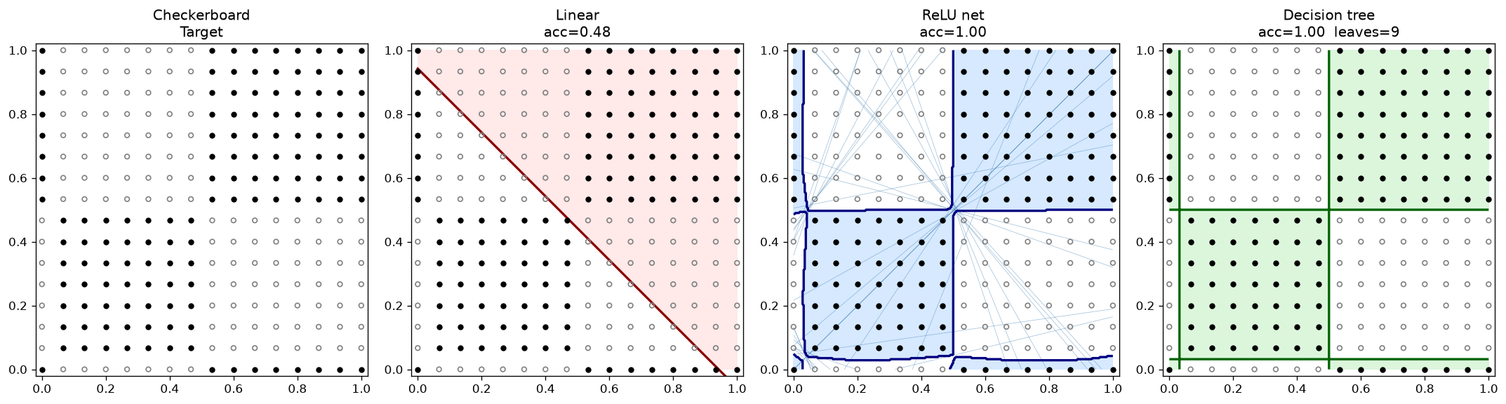
A two-block checkerboard. A linear model is helpless (48% accuracy), while the axis-aligned tree nails it with exactly leaves at . This is the well-aligned regime, where profiles say nothing useful.
Theorem 3 (the general run bound). For every grid labeling,
This is the flagship result, because it proves in full generality the two facts that were previously only conjectured or open:
It also recovers the Theorem 1 lower bound as a special case, since on the triangle gives .
Why runs, and not just profiles
The proof is a strong induction on over the recursive guillotine structure of the tree (an axis-aligned tree is just a recursive sequence of guillotine cuts). The subtlety is what survives a cut parallel to the scan direction. Distinct-profile counts are only sub-multiplicative there, , which is too weak to induct on. Run counts behave far better: they are sub-additive with a gain,
because concatenating two pieces can never manufacture a new adjacency between equal profiles. Summing the inductive bounds across a root cut yields . Strengthening the induction hypothesis from counts to runs is the whole trick.
The bound is tight on the triangle () and on alternating stripes (, where the plain profile bound would give only 2), and it was checked exhaustively by an exact guillotine dynamic program over all 512 labelings of the grid and all 65,536 labelings of the grid.
Three alignment regimes
Putting the theorems together gives a clean picture of when each invariant is the right one.
| Regime | Example | Tight invariant | Status |
|---|---|---|---|
| Poor | Oblique halfspace | proved (tight via Theorem 1) | |
| Good | Checkerboard | cells | proved (Theorem 2) |
| Neutral | Disk | (approximation) | conjectured |
The disk, and what stays open
Smooth targets sit between the two extremes. For a disk at grid resolution , the exact tree complexity is , and the run bound gives , the best rigorous lower bound available but no longer tight.
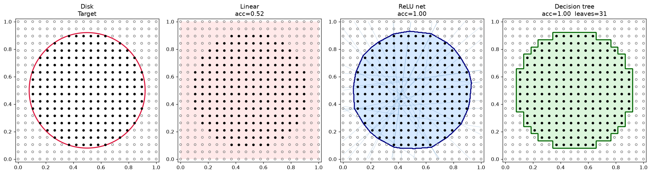
A disk. The greedy tree shown here uses 31 leaves; the exact optimum at this resolution is 29, and the run bound guarantees only 21. Smooth boundaries are the neutral regime, where no simple invariant is tight.
Counting mixed columns and rows (, those that a cut cannot keep pure) approximates closely, and the revised conjecture is that for strictly convex smooth targets. It is worth being honest about what the data says: is neither a lower nor an upper bound. It reads against at , then against at , then against at , erring in both directions. And vertical stripes ( large, ) kill any general lower-bound version outright. So it is an approximation law, not a bound, and proving the two-sided constants is open.
The larger open question is a single invariant that interpolates between the run bound (poor alignment, linear cost) and the cell-count law (good alignment, quadratic cost), and ideally one that lifts to higher dimensions, perhaps as .
Takeaway
Once every mechanism lives on a shared labeled grid, "which model is simpler here" stops being a matter of taste and becomes a matter of counting. Profiles and runs supply the vocabulary, the triangle and checkerboard pin down the two extreme regimes exactly, and the run bound gives one general lower bound that holds for every labeling.