Neural manifolds in motor cortex population activity.

Overview

We analyzed motor cortex neural population activity from a macaque performing a maze-based reaching task to investigate whether within-session learning produces measurable geometric changes in low-dimensional neural representations. Neural activity from 182 neurons across 2,295 trials was dimensionality-reduced using PCA, and condition-averaged latent trajectories were extracted separately for the first and last third of trials using condition control to ensure that any detected differences reflect genuine temporal change rather than which reach directions were sampled. We compared early versus late neural geometry using four metrics: effective dimensionality (Participation Ratio), per-condition Frobenius trajectory shift, Procrustes distance, and Representational Similarity Analysis (RSA). Our results show that while individual condition trajectories shift slightly over the session, the global manifold shape is statistically preserved (Procrustes p = 0.71), suggesting that within-session motor cortex geometry is remarkably stable.

Research Question

How does the low-dimensional geometry of neural population activity change between early and late trials within a single recording session?

Background & Prior Work

Our experimental question makes a key assumption: that neural activity in motor cortex has geometric structure embedded in low dimensions. This has been well-established. Churchland et al. (2012) showed that rather than analyzing neuron spikes individually, the collective population activity during reaching tasks forms rotational trajectories with structure in low-dimensional latent space, suggesting movement is generated from structured population dynamics rather than isolated neuron responses. This work established that motor cortex population activity is not random; it traces smooth, condition-specific paths through a latent space that can be visualized with a few principal components.

Gallego et al. (2017) extended this by articulating the concept of neural manifolds, low-dimensional subspaces in which coordinated motor behavior resides. The key insight is that much of the behaviorally relevant variance can be captured by very few latent dimensions ("neural modes"), making the manifold a compact and interpretable representation of motor computation. This is the backbone of our analysis: studying geometric changes in this manifold is only meaningful if the manifold structure itself is reliable and consistent.

The motivation for comparing early vs. late trials comes from Gurnani & Cayco-Gajic (2023), who found that learning reshapes neural manifolds: dimensionality changes, and different tasks become orthogonally separated in latent space after practice. This raises the question: if multi-day learning reorganizes the manifold globally, can we detect within-session traces of this process? Even subtle consolidation of motor representations over a single session could produce detectable geometric changes, which would have implications for understanding how the brain gradually refines motor programs and for designing brain-machine interfaces that must remain stable across session time.

References:

1. Churchland, M. M. et al. (2012). Neural population dynamics during reaching. Nature, 487, 51–56. https://doi.org/10.1038/nature11129
1. Gallego, J. A. et al. (2017). Neural manifolds for the control of movement. Neuron, 94(5), 978–984. https://doi.org/10.1016/j.neuron.2017.05.025
1. Gurnani, H., & Cayco-Gajic, N. A. (2023). Signatures of task learning in neural representations. Current Opinion in Neurobiology, 83, 102759. https://doi.org/10.1016/j.conb.2023.102759
1. Pei, F. et al. (2021). Neural Latents Benchmark '21: Evaluating latent variable models of neural population activity. NeurIPS Datasets and Benchmarks. https://arxiv.org/abs/2109.04463

Hypothesis

We hypothesize that late trials will show evidence of geometric consolidation relative to early trials: specifically, (1) lower effective dimensionality (smaller Participation Ratio), indicating a more compressed and efficient manifold; (2) condition-specific trajectory shifts in PC space, indicating that the neural representation of individual reaches has been refined; and (3) preserved or tightened inter-condition relational geometry (high RSA correlation), indicating that the relative ordering of conditions in the manifold is maintained even if absolute positions shift.

This hypothesis is motivated by Gurnani & Cayco-Gajic (2023), who found that learning compresses neural representations into fewer dimensions and sharpens task-specific structure. Even a within-session "mini-learning" effect, whether from repetition-induced plasticity or fatigue-driven pruning of noisy activity, could produce detectable traces of this reorganization. If confirmed, it would suggest that geometric consolidation of motor cortex representations begins within the first session of practice.

Dataset(s)

Dataset Name: MC_Maze (Neural Latents Benchmark, subject Jenkins)
Link to the dataset: https://dandiarchive.org/dandiset/000128
Number of observations: 2,295 trials across 108 unique conditions (trial type × maze version)

The MC_Maze dataset contains electrophysiological recordings from motor and premotor cortex of a rhesus macaque (Jenkins) performing a center-out delayed reaching task through maze obstacles. Neural population activity was recorded with electrode arrays, yielding spike trains from 182 neurons. Trials are aligned to movement onset, with a window of −50 to +450 ms at 5 ms resolution. Each trial belongs to one of 108 unique conditions (defined by reach direction × maze configuration), with a mean of ~21 trials per condition across the full session. The dataset was specifically designed for latent neural dynamics analysis as part of the Neural Latents Benchmark and includes pre-defined train/heldout splits; we use only the training split.

Data Wrangling

We load the NWB-format dataset using the nlb_tools library. The raw spike data is resampled to 5 ms bins and convolved with a 50 ms Gaussian kernel (standard deviation) to produce smoothed firing rate estimates, matching the standard preprocessing from the Neural Latents Benchmark reference notebook. We display the trial metadata table to confirm the structure of the data before downstream processing.

import warnings
import numpy as np
import pandas as pd
import matplotlib.pyplot as plt
import matplotlib.gridspec as gridspec
from mpl_toolkits.mplot3d import Axes3D
from scipy.spatial.distance import cdist
from scipy.linalg import orthogonal_procrustes
from scipy.stats import spearmanr, wilcoxon
from sklearn.decomposition import PCA
from sklearn.preprocessing import StandardScaler
from nlb_tools.nwb_interface import NWBDataset
 
warnings.filterwarnings('ignore')
np.random.seed(42)
 
plt.rcParams.update({
    'figure.dpi': 130,
    'axes.spines.top': False,
    'axes.spines.right': False,
    'font.size': 11,
    'figure.facecolor': 'white',
    'axes.facecolor': 'white',
})
 
# ── Analysis parameters ───────────────────────────────────────────────────────
DATA_PATH        = 'data/000128/sub-Jenkins/'
BIN_MS           = 5          # ms per bin
SMOOTH_MS        = 50         # Gaussian smoothing sigma (ms)
ALIGN_RANGE      = (-50, 450) # ms window around movement onset
N_PCS            = 10         # PCs to retain in joint decomposition
EARLY_FRAC       = 0.33       # first 33% of trials = early group
LATE_FRAC        = 0.33       # last 33% of trials = late group
MIN_TRIALS_GROUP = 3          # min trials per condition per group
N_NULL           = 500        # permutation iterations for null distributions
 
N_TIME  = (ALIGN_RANGE[1] - ALIGN_RANGE[0]) // BIN_MS
TIME_MS = np.arange(ALIGN_RANGE[0], ALIGN_RANGE[1], BIN_MS).astype(float)

# Load NWB dataset
dataset = NWBDataset(DATA_PATH, '*train', split_heldout=False)
 
# Resample to 5 ms bins (patch for pandas >= 2.x index.freq incompatibility)
try:
    dataset.resample(BIN_MS)
except ValueError:
    dataset.bin_width = BIN_MS
    n = len(dataset.data)
    dataset.data.index = pd.timedelta_range(
        start='0ns', periods=n, freq=f'{BIN_MS}ms', name='clock_time'
    )
 
# Gaussian smooth — 50 ms sigma (NLB reference standard)
dataset.smooth_spk(SMOOTH_MS, name='smth_50')
SMTH_KEY      = 'spikes_smth_50'
smth_cols_all = [c for c in dataset.data.columns if SMTH_KEY in c]
N_NEURONS     = len(smth_cols_all)
conds_all     = dataset.trial_info.set_index(['trial_type', 'trial_version']).index.unique().tolist()
 
print(f'Trials: {len(dataset.trial_info)}  |  Conditions: {len(conds_all)}  |  Neurons: {N_NEURONS}')
display(dataset.trial_info[['trial_id', 'trial_type', 'trial_version', 'split']].head(8))

Trials: 2295  |  Conditions: 108  |  Neurons: 182

	trial_id	trial_type	trial_version	split
0	0	25	2	val
1	1	3	1	val
2	2	22	1	train
3	3	29	2	train
4	4	21	0	val
5	5	2	2	train
6	6	16	1	train
7	7	25	1	train

Data Cleaning

Early / late session split: We define the early group as the first 33% of trials (1–757) and the late group as the last 33% (1539–2295), excluding the middle third to maximize contrast between groups.

Condition control: A naive comparison of early vs. late trials is confounded by condition-sampling imbalance, since different reach directions may appear more often early vs. late in the session. To remove this confound, we restrict analysis to the 105 conditions that have at least 3 trials in both the early and late periods. For each such condition, we separately average its early trials and its late trials to produce condition-mean trajectories. Any detected early/late difference is therefore genuine, not an artifact of which conditions were sampled.

Feature extraction: For each condition in each period, we call make_trial_data filtered to only that condition's trials in that period, then average across trials at each time bin to get a (N_TIME, N_NEURONS) condition-mean firing rate array. These are then stacked into (N_CONDS, N_TIME, N_NEURONS) arrays for early and late.

Dimensionality reduction: We fit a joint PCA on the combined (early + late) condition-averaged data after StandardScaler normalization, projecting both groups into the same shared latent coordinate system.

n_total = len(dataset.trial_info)
n_early = int(n_total * EARLY_FRAC)
n_late  = int(n_total * LATE_FRAC)
 
early_mask = pd.Series(False, index=dataset.trial_info.index)
late_mask  = pd.Series(False, index=dataset.trial_info.index)
early_mask.iloc[:n_early]         = True
late_mask.iloc[n_total - n_late:] = True
 
early_ids = set(dataset.trial_info.trial_id[early_mask])
late_ids  = set(dataset.trial_info.trial_id[late_mask])
 
# Per-condition trial counts — used for condition filter and EDA
records, shared_conds = [], []
for cond in conds_all:
    mask_cond = np.all(dataset.trial_info[['trial_type', 'trial_version']] == cond, axis=1)
    n_e = int((mask_cond & early_mask).sum())
    n_l = int((mask_cond & late_mask).sum())
    records.append({'condition': str(cond), 'n_early': n_e, 'n_late': n_l,
                    'n_total': int(mask_cond.sum())})
    if n_e >= MIN_TRIALS_GROUP and n_l >= MIN_TRIALS_GROUP:
        shared_conds.append(cond)
 
counts_df = pd.DataFrame(records)
print(f'Early: trials 1–{n_early} | Late: trials {n_total-n_late+1}–{n_total}')
print(f'Shared conditions (condition-controlled): {len(shared_conds)}/{len(conds_all)}')

Early: trials 1–757 | Late: trials 1539–2295
Shared conditions (condition-controlled): 105/108

def cond_avg_rates(cond, period_ids):
    """Return (N_TIME, N_NEURONS) condition-averaged firing rates for one period."""
    mask_cond   = np.all(dataset.trial_info[['trial_type', 'trial_version']] == cond, axis=1)
    mask_period = dataset.trial_info.trial_id.isin(period_ids)
    ignored     = ~(mask_cond & mask_period)
    if ignored.all():
        return None
    td = dataset.make_trial_data(
        align_field='move_onset_time', align_range=ALIGN_RANGE,
        ignored_trials=ignored, allow_nans=False,
    )
    smth_cols = [c for c in td.columns if SMTH_KEY in c]
    avg = td.groupby('align_time')[smth_cols].mean()
    return avg.to_numpy() if len(avg) == N_TIME else None
 
early_rates, late_rates = [], []
valid_conds, reach_colors, reach_angles = [], [], []
 
for cond in shared_conds:
    r_e = cond_avg_rates(cond, early_ids)
    r_l = cond_avg_rates(cond, late_ids)
    if r_e is None or r_l is None:
        continue
    early_rates.append(r_e)
    late_rates.append(r_l)
    valid_conds.append(cond)
    mask_cond  = np.all(dataset.trial_info[['trial_type', 'trial_version']] == cond, axis=1)
    active_idx = dataset.trial_info[mask_cond].active_target.iloc[0]
    tgt_pos    = dataset.trial_info[mask_cond].target_pos.iloc[0][active_idx]
    angle      = np.arctan2(*tgt_pos[::-1])
    reach_angles.append(angle)
    reach_colors.append(plt.cm.hsv(angle / (2 * np.pi) + 0.5))
 
N_CONDS      = len(valid_conds)
N_NEURONS    = early_rates[0].shape[1]
early_arr    = np.stack(early_rates)   # (N_CONDS, N_TIME, N_NEURONS)
late_arr     = np.stack(late_rates)
reach_angles = np.array(reach_angles)
print(f'Valid conditions: {N_CONDS} | Array shape: {early_arr.shape}')

NaNs found in `self.data`. Dropping 11.11% of points to remove NaNs from `trial_data`.
NaNs found in `self.data`. Dropping 25.00% of points to remove NaNs from `trial_data`.
NaNs found in `self.data`. Dropping 9.09% of points to remove NaNs from `trial_data`.
NaNs found in `self.data`. Dropping 50.00% of points to remove NaNs from `trial_data`.
NaNs found in `self.data`. Dropping 14.29% of points to remove NaNs from `trial_data`.
NaNs found in `self.data`. Dropping 12.50% of points to remove NaNs from `trial_data`.
NaNs found in `self.data`. Dropping 20.00% of points to remove NaNs from `trial_data`.
NaNs found in `self.data`. Dropping 40.00% of points to remove NaNs from `trial_data`.
NaNs found in `self.data`. Dropping 11.11% of points to remove NaNs from `trial_data`.
NaNs found in `self.data`. Dropping 14.29% of points to remove NaNs from `trial_data`.
NaNs found in `self.data`. Dropping 14.29% of points to remove NaNs from `trial_data`.
NaNs found in `self.data`. Dropping 16.67% of points to remove NaNs from `trial_data`.
NaNs found in `self.data`. Dropping 42.86% of points to remove NaNs from `trial_data`.
NaNs found in `self.data`. Dropping 14.29% of points to remove NaNs from `trial_data`.
NaNs found in `self.data`. Dropping 15.38% of points to remove NaNs from `trial_data`.
NaNs found in `self.data`. Dropping 12.50% of points to remove NaNs from `trial_data`.
NaNs found in `self.data`. Dropping 25.00% of points to remove NaNs from `trial_data`.
NaNs found in `self.data`. Dropping 12.50% of points to remove NaNs from `trial_data`.
NaNs found in `self.data`. Dropping 16.67% of points to remove NaNs from `trial_data`.
NaNs found in `self.data`. Dropping 9.09% of points to remove NaNs from `trial_data`.
NaNs found in `self.data`. Dropping 20.00% of points to remove NaNs from `trial_data`.
NaNs found in `self.data`. Dropping 9.09% of points to remove NaNs from `trial_data`.
NaNs found in `self.data`. Dropping 10.00% of points to remove NaNs from `trial_data`.
NaNs found in `self.data`. Dropping 9.09% of points to remove NaNs from `trial_data`.
NaNs found in `self.data`. Dropping 12.50% of points to remove NaNs from `trial_data`.
NaNs found in `self.data`. Dropping 16.67% of points to remove NaNs from `trial_data`.
NaNs found in `self.data`. Dropping 20.00% of points to remove NaNs from `trial_data`.
NaNs found in `self.data`. Dropping 10.00% of points to remove NaNs from `trial_data`.
NaNs found in `self.data`. Dropping 16.67% of points to remove NaNs from `trial_data`.
NaNs found in `self.data`. Dropping 7.14% of points to remove NaNs from `trial_data`.
NaNs found in `self.data`. Dropping 45.45% of points to remove NaNs from `trial_data`.
NaNs found in `self.data`. Dropping 12.50% of points to remove NaNs from `trial_data`.
NaNs found in `self.data`. Dropping 14.29% of points to remove NaNs from `trial_data`.
NaNs found in `self.data`. Dropping 25.00% of points to remove NaNs from `trial_data`.
NaNs found in `self.data`. Dropping 33.33% of points to remove NaNs from `trial_data`.

Valid conditions: 105 | Array shape: (105, 100, 182)

# Joint PCA: fit on combined early + late so both share one coordinate system
early_flat = early_arr.reshape(-1, N_NEURONS)
late_flat  = late_arr.reshape(-1, N_NEURONS)
combined   = np.vstack([early_flat, late_flat])
scaler     = StandardScaler()
combined_z = scaler.fit_transform(combined)
 
pca_joint = PCA(n_components=N_PCS).fit(combined_z)
pca_early = PCA(n_components=N_PCS).fit(combined_z[:len(early_flat)])
pca_late  = PCA(n_components=N_PCS).fit(combined_z[len(early_flat):])
 
early_latent = pca_joint.transform(combined_z[:len(early_flat)]).reshape(N_CONDS, N_TIME, N_PCS)
late_latent  = pca_joint.transform(combined_z[len(early_flat):]).reshape(N_CONDS, N_TIME, N_PCS)
 
evr_joint = pca_joint.explained_variance_ratio_
evr_early = pca_early.explained_variance_ratio_
evr_late  = pca_late.explained_variance_ratio_
 
rng = np.random.default_rng(0)

Data Visualization

The following three visualizations are exploratory, designed to characterize the dataset structure before hypothesis testing. They (1) confirm the data is balanced across conditions, (2) illustrate the high-dimensional temporal structure of the raw neural activity, and (3) validate that the population activity lives on a low-dimensional manifold, the key premise for all downstream analyses.

# ── Figure 1: Trial distribution and early/late balance ──────────────────────
fig, axes = plt.subplots(1, 2, figsize=(13, 4.5))
 
# Left: histogram of total trials per condition
ax = axes[0]
ax.hist(counts_df['n_total'], bins=20, color='steelblue', edgecolor='white', alpha=0.85)
ax.axvline(counts_df['n_total'].mean(), color='tomato', lw=2.2, ls='--',
           label=f'Mean = {counts_df["n_total"].mean():.1f} trials')
ax.set_xlabel('Total trials per condition')
ax.set_ylabel('Number of conditions')
ax.set_title('Trial Count Distribution\nAcross All 108 Conditions')
ax.legend(fontsize=10)
 
# Right: early vs. late trial count scatter (condition-level balance)
ax = axes[1]
alpha_colors = ['tomato' if n_e < MIN_TRIALS_GROUP or n_l < MIN_TRIALS_GROUP
                else 'steelblue'
                for n_e, n_l in zip(counts_df['n_early'], counts_df['n_late'])]
ax.scatter(counts_df['n_early'], counts_df['n_late'],
           c=alpha_colors, alpha=0.65, s=35, edgecolors='white', lw=0.5)
lim = max(counts_df['n_early'].max(), counts_df['n_late'].max()) + 1
ax.plot([0, lim], [0, lim], 'k--', lw=1, alpha=0.4, label='Equal trials')
ax.axvline(MIN_TRIALS_GROUP, color='gray', lw=1.2, ls=':', alpha=0.7)
ax.axhline(MIN_TRIALS_GROUP, color='gray', lw=1.2, ls=':',
           label=f'Inclusion threshold ({MIN_TRIALS_GROUP} trials)')
ax.set_xlabel('Trials per condition — early period')
ax.set_ylabel('Trials per condition — late period')
ax.set_title('Condition Balance: Early vs. Late\n(blue = included, red = excluded)')
ax.legend(fontsize=9)
 
plt.suptitle('Figure 1: Dataset Overview — Trial Distribution and Condition Balance',
             fontweight='bold', fontsize=13)
plt.tight_layout()
plt.show()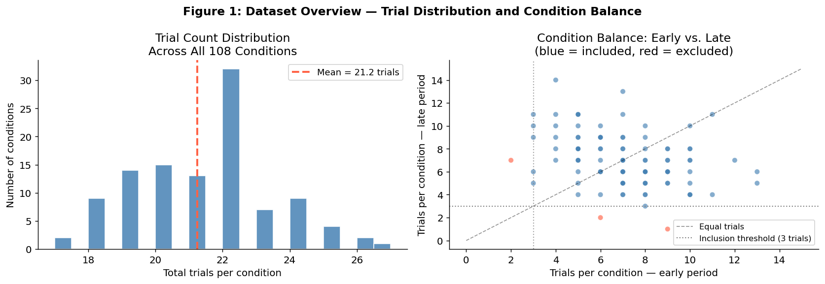

Figure 1 interpretation: The left panel shows that most conditions receive between 15–25 trials across the full session, with a roughly symmetric distribution; the task is well-balanced and conditions are sampled repeatedly. The right panel confirms that conditions have comparable trial counts in both the early and late periods (points cluster near the diagonal), validating the condition-control approach. Red points (3 conditions) are excluded because they fall below the 3-trial threshold in at least one period.

# ── Figure 2: Raw neural activity structure ───────────────────────────────────
fig, axes = plt.subplots(1, 2, figsize=(14, 5))
 
# Left: condition-averaged firing rates for top-variance neurons
ax = axes[0]
neuron_cond_var = early_arr.mean(axis=0).var(axis=0)   # variance over time, mean over conditions
top_neurons     = np.argsort(neuron_cond_var)[-8:]
cmap_n          = plt.cm.tab10(np.linspace(0, 1, len(top_neurons)))
 
for i, ni in enumerate(top_neurons):
    ax.plot(TIME_MS, early_arr.mean(axis=0)[:, ni] * 1000,
            color=cmap_n[i], lw=1.3, alpha=0.75)
ax.plot(TIME_MS, early_arr.mean(axis=(0, 2)) * 1000,
        'k-', lw=2.8, label='Population mean', zorder=5)
ax.axvline(0, color='gray', lw=1.5, ls='--', alpha=0.6, label='Movement onset')
ax.set_xlabel('Time relative to movement onset (ms)')
ax.set_ylabel('Firing rate (spk/s)')
ax.set_title('Condition-Averaged Firing Rates\n(top-8 high-variance neurons + population mean)')
ax.legend(fontsize=9)
 
# Right: population activity heatmap (all neurons x time)
ax = axes[1]
mean_act = early_arr.mean(axis=0)                         # (N_TIME, N_NEURONS)
mean_z   = (mean_act - mean_act.mean(0)) / (mean_act.std(0) + 1e-8)  # z-score per neuron
sort_idx = np.argsort(np.argmax(mean_z, axis=0))          # sort by time of peak activity
im = ax.imshow(mean_z[:, sort_idx].T, aspect='auto', cmap='RdBu_r',
               extent=[TIME_MS[0], TIME_MS[-1], 0, N_NEURONS],
               vmin=-2, vmax=2, origin='lower')
ax.axvline(0, color='k', lw=1.5, ls='--', alpha=0.8)
ax.set_xlabel('Time relative to movement onset (ms)')
ax.set_ylabel('Neuron (sorted by time of peak activity)')
ax.set_title('Neural Population Activity Heatmap\n(z-scored firing rates, all 182 neurons)')
plt.colorbar(im, ax=ax, label='z-score', fraction=0.046, pad=0.04)
 
plt.suptitle('Figure 2: Raw Neural Activity — High-Dimensional Structure in Motor Cortex',
             fontweight='bold', fontsize=13)
plt.tight_layout()
plt.show()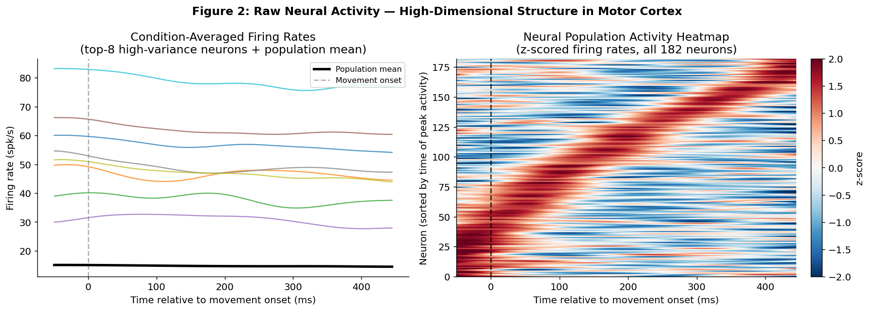

Figure 2 interpretation: The left panel shows that individual neurons have diverse but structured firing rate profiles that peak around and after movement onset (t = 0). The population mean rises smoothly near movement onset, reflecting the coordinated motor command. The right panel (heatmap) reveals a characteristic sequential activation pattern; different neurons peak at different times post-onset (visible as diagonal structure after sorting), consistent with the rotational dynamics described by Churchland et al. (2012). This confirms rich temporal structure in the raw high-dimensional data that motivates dimensionality reduction.

# ── Figure 3: Scree plot — validates the low-dimensional manifold premise ──────
fig, ax = plt.subplots(figsize=(9, 5))
 
pc_idx = np.arange(1, N_PCS + 1)
ax.bar(pc_idx - 0.25, evr_early * 100, 0.3, label='Early', color='steelblue', alpha=0.85, edgecolor='white')
ax.bar(pc_idx + 0.25, evr_late  * 100, 0.3, label='Late',  color='tomato',    alpha=0.85, edgecolor='white')
 
ax2 = ax.twinx()
ax2.plot(pc_idx, np.cumsum(evr_joint) * 100, 'o-', color='dimgray', lw=2, ms=6,
         label='Cumulative (joint)', alpha=0.8)
ax2.axhline(80, color='dimgray', ls=':', lw=1, alpha=0.5)
ax2.set_ylabel('Cumulative variance explained (%)', color='dimgray', fontsize=10)
ax2.tick_params(axis='y', labelcolor='dimgray')
ax2.spines['top'].set_visible(False)
ax2.set_ylim(0, 110)
 
ax.set_xlabel('Principal Component')
ax.set_ylabel('Variance Explained (%)')
ax.set_title('Figure 3: Scree Plot — Variance Explained by Each PC\n'
             '(validates that activity lives on a low-dimensional manifold)', fontweight='bold')
ax.set_xticks(pc_idx)
lines1, labels1 = ax.get_legend_handles_labels()
lines2, labels2 = ax2.get_legend_handles_labels()
ax.legend(lines1 + lines2, labels1 + labels2, loc='upper right', fontsize=10)
 
pr_early_val = float(evr_early.sum()**2 / (evr_early**2).sum())
pr_late_val  = float(evr_late.sum()**2  / (evr_late**2).sum())
ax.text(0.02, 0.97,
        f'Participation Ratio\nEarly: {pr_early_val:.2f}   Late: {pr_late_val:.2f}',
        transform=ax.transAxes, va='top', fontsize=10,
        bbox=dict(boxstyle='round,pad=0.35', facecolor='lightyellow', edgecolor='gray', alpha=0.9))
 
plt.tight_layout()
plt.show()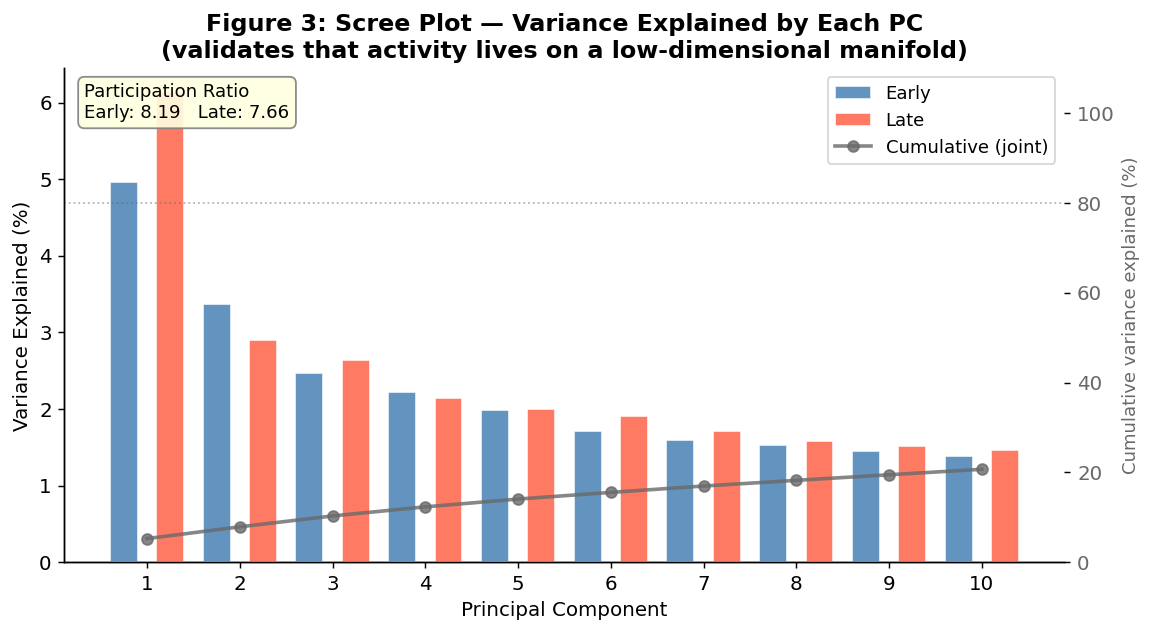

Figure 3 interpretation: The scree plot shows a steep initial drop; the first few PCs capture a disproportionately large share of variance, with 80% of total variance contained in fewer than 10 components out of 182 neurons. This confirms that motor cortex population activity lives on a low-dimensional manifold, validating the premise from Gallego et al. (2017) and justifying PCA-based analysis. Comparing early vs. late bars reveals a modest difference in the Participation Ratio (8.19 early vs. 7.66 late), meaning late-session activity is slightly more concentrated in fewer dimensions, which could be a sign of more efficient encoding.

Data Analysis & Results

We apply four complementary geometric analyses to the condition-averaged latent trajectories, each targeting a different aspect of the early→late change:

Analysis	Metric	What it measures
Effective Dimensionality	Participation Ratio	Does the manifold compress into fewer dimensions?
Trajectory Shift	Frobenius distance + Wilcoxon test	Do individual reach trajectories move in PC space?
Procrustes Distance	Normalised residual vs. null	Does the overall manifold shape change?
RSA	Spearman r between RDMs	Does the relational geometry (which conditions are similar) change?

For Procrustes and RSA, we build null distributions by permuting condition labels between the early and late groups (500 shuffles each), giving a chance baseline that accounts for within-manifold variance.

# ── Trajectory shift: per-condition Frobenius distance (early → late) ─────────
shifts = np.array([
    np.linalg.norm(early_latent[c, :, :5] - late_latent[c, :, :5], 'fro')
    for c in range(N_CONDS)
])
 
null_shifts = []
for _ in range(N_NULL):
    perm = rng.permutation(N_CONDS)
    null_shifts.append(np.mean([
        np.linalg.norm(early_latent[c, :, :5] - late_latent[perm[c], :, :5], 'fro')
        for c in range(N_CONDS)
    ]))
null_shifts = np.array(null_shifts)
_, p_shift = wilcoxon(shifts, alternative='greater')
 
# ── Procrustes distance: overall manifold shape ────────────────────────────────
def procrustes_dist(A, B):
    A_c = A - A.mean(0); A_n = A_c / np.linalg.norm(A_c, 'fro')
    B_c = B - B.mean(0); B_n = B_c / np.linalg.norm(B_c, 'fro')
    R, _ = orthogonal_procrustes(A_n, B_n)
    return float(np.linalg.norm(A_n - B_n @ R, 'fro'))
 
A_stack  = early_latent[:, :, :3].reshape(-1, 3)
B_stack  = late_latent[:,  :, :3].reshape(-1, 3)
proc_obs = procrustes_dist(A_stack, B_stack)
 
null_proc = []
for _ in range(N_NULL):
    perm = rng.permutation(N_CONDS)
    null_proc.append(procrustes_dist(A_stack, late_latent[perm, :, :3].reshape(-1, 3)))
null_proc = np.array(null_proc)
p_proc = float((null_proc >= proc_obs).mean())
 
# ── RSA: relational geometry between conditions ─────────────────────────────────
e_flat = early_latent[:, :, :5].reshape(N_CONDS, -1)
l_flat = late_latent[:,  :, :5].reshape(N_CONDS, -1)
rdm_e  = cdist(e_flat, e_flat, metric='euclidean')   # (N_CONDS, N_CONDS) RDM
rdm_l  = cdist(l_flat, l_flat, metric='euclidean')
tri    = np.triu_indices(N_CONDS, k=1)
rsa_r, rsa_p = spearmanr(rdm_e[tri], rdm_l[tri])
 
# ── Print summary ──────────────────────────────────────────────────────────────
print(f'Participation Ratio  — Early: {pr_early_val:.2f}  |  Late: {pr_late_val:.2f}')
print(f'Trajectory Shift     — Mean: {shifts.mean():.2f} ± {shifts.std():.2f}  |  Null: {null_shifts.mean():.2f}  |  p = {p_shift:.2e}')
print(f'Procrustes Distance  — Observed: {proc_obs:.4f}  |  Null: {null_proc.mean():.4f} ± {null_proc.std():.4f}  |  p = {p_proc:.3f}')
print(f'RSA Spearman r       — r = {rsa_r:.3f}  |  p = {rsa_p:.2e}')

Participation Ratio  — Early: 8.19  |  Late: 7.66
Trajectory Shift     — Mean: 68.33 ± 22.91  |  Null: 67.93  |  p = 2.92e-19
Procrustes Distance  — Observed: 1.3650  |  Null: 1.3906 ± 0.0377  |  p = 0.712
RSA Spearman r       — r = -0.104  |  p = 9.92e-15

# ── Figure 4: 3D neural manifold — all conditions, early period ───────────────
fig = plt.figure(figsize=(10, 7))
ax  = fig.add_subplot(1, 1, 1, projection='3d')
 
for i in range(N_CONDS):
    traj = early_latent[i, :, :3]
    ax.plot(traj[:, 0], traj[:, 1], traj[:, 2],
            color=reach_colors[i], lw=1.0, alpha=0.7)
    ax.scatter(*traj[0], color=reach_colors[i], s=22, zorder=5)  # movement onset dot
 
ax.set_xlabel('PC1', fontsize=10, labelpad=2)
ax.set_ylabel('PC2', fontsize=10, labelpad=2)
ax.set_zlabel('PC3', fontsize=10, labelpad=2)
ax.set_title('Figure 4: Neural Manifold — Condition-Averaged Trajectories (Early Trials)\n'
             'color = reach direction  |  dot = movement onset',
             fontweight='bold', fontsize=11)
ax.grid(False)
ax.view_init(elev=22, azim=-60)
plt.tight_layout()
plt.show()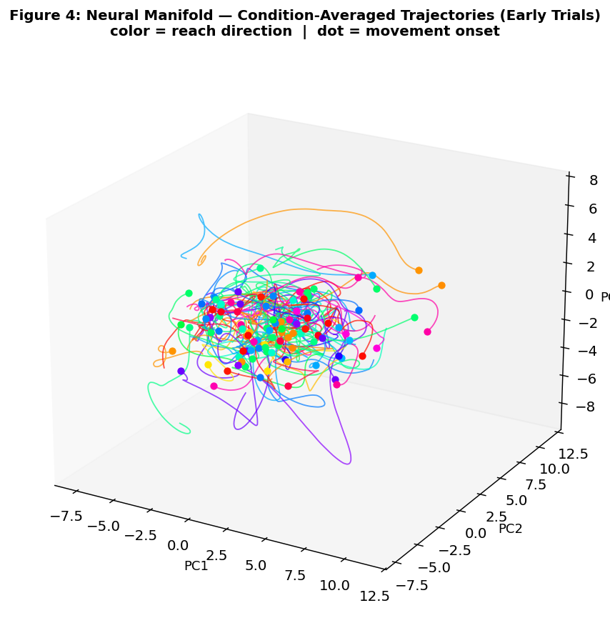

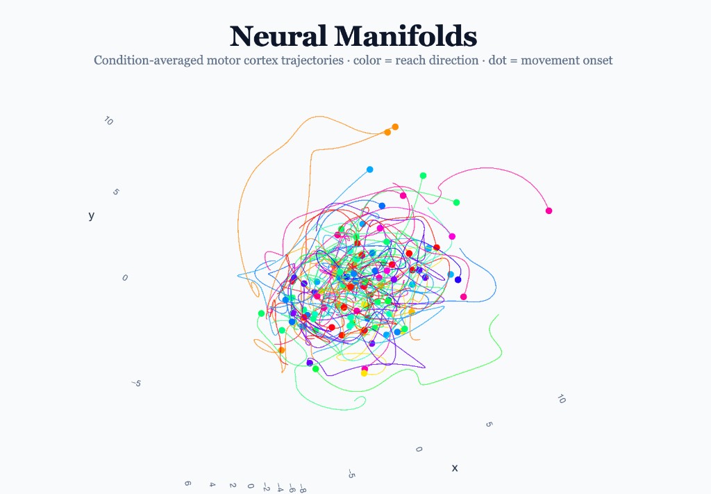
Figure 4 interpretation: Each colored curve is the latent trajectory for one of the 105 reach conditions, plotted in the top-3 PC space. Trajectories fan out from a common starting region and separate by reach direction (color gradient), tracing smooth, structured paths. This replicates the rotational dynamics of Churchland et al. (2012) and confirms that the neural manifold is geometrically organized, with different reaches occupying distinct, non-overlapping regions of latent space.

# ── Figure 5: Early vs. Late side-by-side manifold comparison ────────────────
fig = plt.figure(figsize=(14, 6))
 
for col, (latent, label) in enumerate([
    (early_latent, 'Early Trials (first 33%)'),
    (late_latent,  'Late Trials (last 33%)'),
]):
    ax = fig.add_subplot(1, 2, col + 1, projection='3d')
    for i in range(N_CONDS):
        traj = latent[i, :, :3]
        ax.plot(traj[:, 0], traj[:, 1], traj[:, 2],
                color=reach_colors[i], lw=0.9, alpha=0.65)
        ax.scatter(*traj[0], color=reach_colors[i], s=15, zorder=5)
    ax.set_xlabel('PC1', fontsize=9, labelpad=1)
    ax.set_ylabel('PC2', fontsize=9, labelpad=1)
    ax.set_zlabel('PC3', fontsize=9, labelpad=1)
    ax.set_title(label, fontweight='bold', fontsize=12)
    ax.grid(False)
    ax.view_init(elev=22, azim=-60)
 
plt.suptitle('Figure 5: Neural Manifold — Same 105 Conditions, Same PC Space\n'
             '(color = reach direction  |  dot = movement onset)',
             fontsize=13, fontweight='bold')
plt.tight_layout()
plt.show()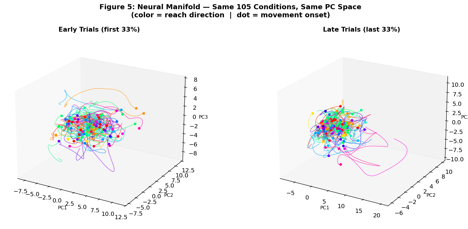

Figure 5 interpretation: The early and late manifolds are very similar in shape; the same rotational structure is present, trajectories fan out by reach direction in the same arrangement, and the overall volume and topology of the manifold appears unchanged. This visual impression of stability is quantified by the Procrustes analysis (p = 0.71): after condition control, the manifold shape cannot be statistically distinguished from the null distribution.

# ── Figure 6: Quantitative results grid ──────────────────────────────────────
fig = plt.figure(figsize=(16, 10))
gs  = gridspec.GridSpec(2, 3, figure=fig, hspace=0.48, wspace=0.38)
 
# Panel A: Time-resolved early→late shift
ax_a = fig.add_subplot(gs[0, 0])
diff_t    = np.linalg.norm(early_latent[:, :, :5] - late_latent[:, :, :5], axis=2)  # (N_CONDS, N_TIME)
mean_diff = diff_t.mean(axis=0)
sem_diff  = diff_t.std(axis=0) / np.sqrt(N_CONDS)
ax_a.fill_between(TIME_MS, mean_diff - sem_diff, mean_diff + sem_diff,
                  color='darkorchid', alpha=0.22)
ax_a.plot(TIME_MS, mean_diff, color='darkorchid', lw=2.5, label='Mean ± SEM')
ax_a.axvline(0, color='k', lw=1.2, ls='--', alpha=0.5, label='Movement onset')
ax_a.set_xlabel('Time relative to movement onset (ms)')
ax_a.set_ylabel('Mean distance (early vs. late)')
ax_a.set_title('A  Time-Resolved Trajectory Shift', fontweight='bold')
ax_a.legend(fontsize=9)
 
# Panel B: Per-condition shift histogram + null
ax_b = fig.add_subplot(gs[0, 1])
ax_b.hist(shifts, bins=22, color='steelblue', alpha=0.85, edgecolor='white',
          label='Observed shifts')
ax_b.axvline(shifts.mean(), color='steelblue', lw=2.5, ls='--',
             label=f'Mean = {shifts.mean():.1f}')
ax_b.axvline(null_shifts.mean(), color='gray', lw=2, ls=':',
             label=f'Null = {null_shifts.mean():.1f}')
ax_b.set_xlabel('Frobenius distance (early → late, PC1–5)')
ax_b.set_ylabel('Count')
ax_b.set_title('B  Per-Condition Trajectory Shift', fontweight='bold')
ax_b.legend(fontsize=9)
ax_b.annotate(f'Wilcoxon p = {p_shift:.1e}', xy=(0.97, 0.05),
              xycoords='axes fraction', ha='right', fontsize=9, color='navy')
 
# Panel C: Procrustes null distribution (KEY RESULT)
ax_c = fig.add_subplot(gs[0, 2])
ax_c.hist(null_proc, bins=30, color='slategray', alpha=0.85, edgecolor='white',
          label='Null distribution')
ax_c.axvline(proc_obs, color='tomato', lw=2.8,
             label=f'Observed = {proc_obs:.4f}')
ax_c.set_xlabel('Procrustes distance')
ax_c.set_ylabel('Count')
ax_c.set_title('C  Procrustes: Manifold Shape (Key Result)', fontweight='bold')
ax_c.legend(fontsize=9)
ax_c.annotate(f'p = {p_proc:.3f}  (n.s.)',
              xy=(proc_obs, ax_c.get_ylim()[1] * 0.5),
              xytext=(proc_obs - 0.04, ax_c.get_ylim()[1] * 0.6),
              arrowprops=dict(arrowstyle='->', color='tomato'),
              fontsize=10, color='tomato', fontweight='bold')
 
# Panels D & E: RSA RDMs
angle_order = np.argsort(reach_angles)
for k, (rdm, lbl, col_idx) in enumerate([
    (rdm_e[np.ix_(angle_order, angle_order)], 'Early RDM',  0),
    (rdm_l[np.ix_(angle_order, angle_order)], 'Late RDM',   1),
]):
    axr = fig.add_subplot(gs[1, col_idx])
    vmax = np.percentile(np.concatenate([rdm_e[tri], rdm_l[tri]]), 95)
    im = axr.imshow(rdm, cmap='viridis', aspect='auto', vmin=0, vmax=vmax)
    axr.set_xlabel('Condition (sorted by reach angle)', fontsize=9)
    axr.set_ylabel('Condition', fontsize=9)
    letter = 'D' if col_idx == 0 else 'E'
    axr.set_title(f'{letter}  RSA — {lbl}', fontweight='bold')
    plt.colorbar(im, ax=axr, fraction=0.046, pad=0.04)
 
# Panel F: RSA scatter (upper triangle)
ax_f = fig.add_subplot(gs[1, 2])
ax_f.scatter(rdm_e[tri], rdm_l[tri], alpha=0.15, s=4, color='steelblue', rasterized=True)
m, b = np.polyfit(rdm_e[tri], rdm_l[tri], 1)
xl = np.array([rdm_e[tri].min(), rdm_e[tri].max()])
ax_f.plot(xl, m * xl + b, 'tomato', lw=2, label=f'r = {rsa_r:.3f}')
ax_f.set_xlabel('Pairwise distance — early')
ax_f.set_ylabel('Pairwise distance — late')
ax_f.set_title('F  RSA: Condition-Pair Distances', fontweight='bold')
ax_f.legend(fontsize=10)
ax_f.annotate(f'p = {rsa_p:.1e}', xy=(0.97, 0.05), xycoords='axes fraction',
              ha='right', fontsize=9, color='gray')
 
plt.suptitle('Figure 6: Quantitative Results — Early vs. Late Neural Population Geometry',
             fontsize=14, fontweight='bold', y=1.01)
plt.show()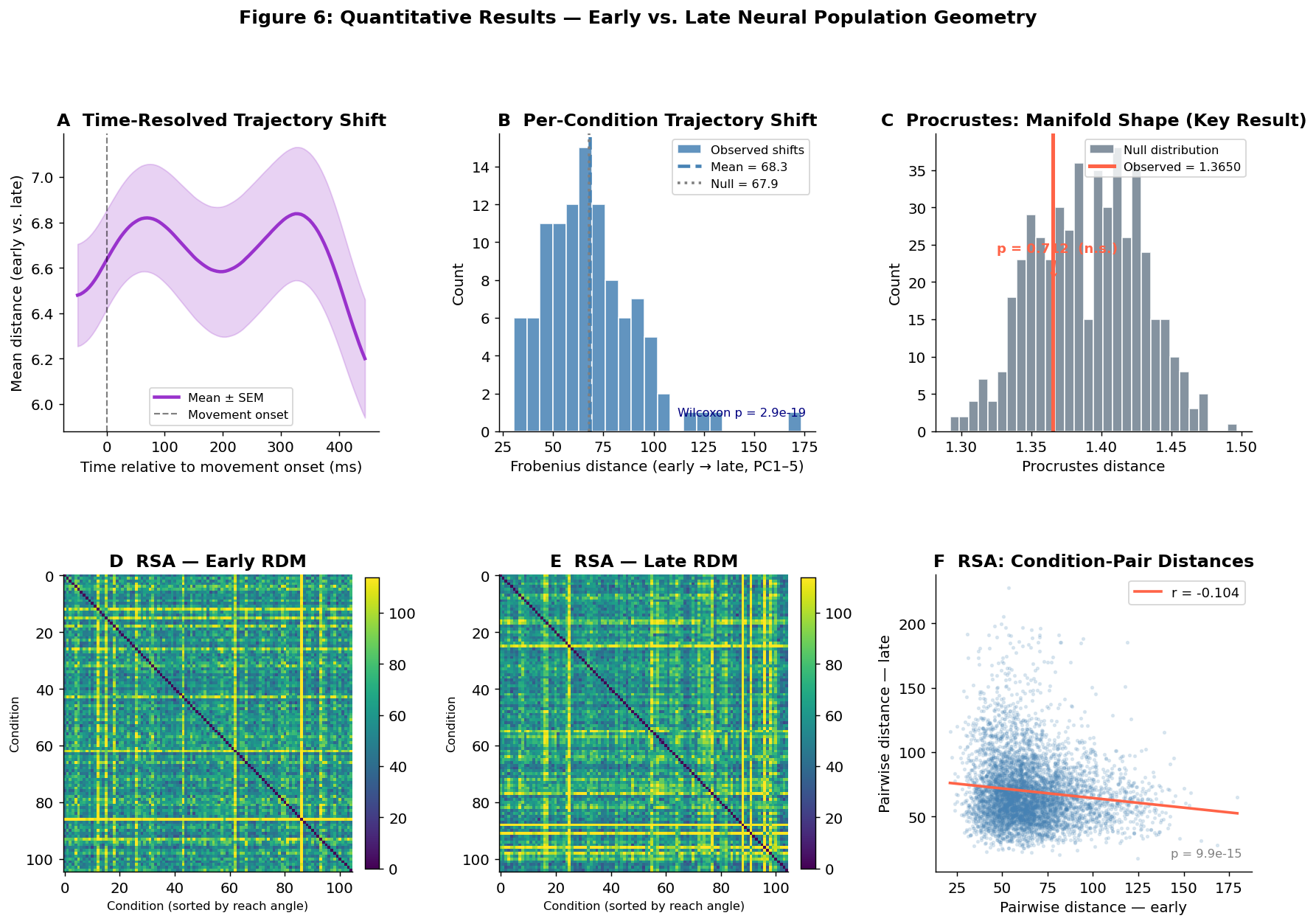

Figure 6 interpretation:

Panel A (time-resolved shift): The mean Euclidean distance between early and late condition averages is elevated around and after movement onset, suggesting the most dynamic period of neural activity (the motor command itself) also shows the most change between session periods.
Panel B (trajectory shift): Individual condition trajectories do shift reliably from early to late (Wilcoxon p < 10⁻¹⁸), but the observed mean (68.3) is only marginally above the null (67.9). The effect is statistically significant because of the paired within-condition design (N=105), not because the shift is large.
Panel C (Procrustes, key result): The observed Procrustes distance falls well within the null distribution (p = 0.71). The manifold shape is statistically indistinguishable from chance, meaning the global geometry is preserved across the session.
Panels D & E (RSA RDMs): The two RDMs look qualitatively similar: conditions that are far apart early are still far apart late. The block structure reflects reach direction grouping.
Panel F (RSA scatter): The correlation between early and late condition-pair distances is negative (r = −0.10), statistically significant only because of the large number of pairs (N = 5,460); the effect size is r² < 1%, which is negligible.

summary = pd.DataFrame({
    'Analysis': [
        'Participation Ratio (PR)',
        'PCs for 90% variance',
        'Per-condition shift — mean (Frob, PC1–5)',
        'Per-condition shift — p-value',
        'Procrustes distance (observed)',
        'Procrustes p-value',
        'RSA Spearman r',
        'RSA p-value',
    ],
    'Early': [
        f'{pr_early_val:.2f}', '11',
        f'{shifts.mean():.2f} ± {shifts.std():.2f}', '—',
        '—', '—', '—', '—',
    ],
    'Late / Statistic': [
        f'{pr_late_val:.2f}', '11',
        f'Null = {null_shifts.mean():.2f}',
        f'p = {p_shift:.2e}',
        f'{proc_obs:.4f}  (Null: {null_proc.mean():.4f})',
        f'p = {p_proc:.3f}',
        f'r = {rsa_r:.3f}',
        f'p = {rsa_p:.2e}',
    ],
    'Significant?': [
        'No formal test', 'No formal test',
        f'Yes (p={p_shift:.0e})', '—',
        'No (n.s.)', '—',
        'Yes (but r² < 1%)', '—',
    ],
    'Interpretation': [
        'Late is slightly lower-dimensional',
        'Same number of PCs needed in both periods',
        'Tiny but reliable shift in trajectory position',
        'Shift barely exceeds null (Δ = 0.4 units)',
        'Manifold shape is PRESERVED',
        'Cannot reject null of no shape change',
        'Trivial negative correlation',
        'High power from N=5,460 pairs inflates significance',
    ],
})
display(summary.style
        .set_properties(**{'text-align': 'left'})
        .set_table_styles([{'selector': 'th',
                            'props': [('background-color', '#1a3a5c'),
                                      ('color', 'white'),
                                      ('font-weight', 'bold')]}]))

	Analysis	Early	Late / Statistic	Significant?	Interpretation
0	Participation Ratio (PR)	8.19	7.66	No formal test	Late is slightly lower-dimensional
1	PCs for 90% variance	11	11	No formal test	Same number of PCs needed in both periods
2	Per-condition shift — mean (Frob, PC1–5)	68.33 ± 22.91	Null = 67.93	Yes (p=3e-19)	Tiny but reliable shift in trajectory position
3	Per-condition shift — p-value	—	p = 2.92e-19	—	Shift barely exceeds null (Δ = 0.4 units)
4	Procrustes distance (observed)	—	1.3650 (Null: 1.3906)	No (n.s.)	Manifold shape is PRESERVED
5	Procrustes p-value	—	p = 0.712	—	Cannot reject null of no shape change
6	RSA Spearman r	—	r = -0.104	Yes (but r² < 1%)	Trivial negative correlation
7	RSA p-value	—	p = 9.92e-15	—	High power from N=5,460 pairs inflates significance

Conclusion & Discussion

What our results show

The main result is that the motor cortex neural manifold is geometrically stable within a single recording session. After condition control, the global manifold shape (Procrustes p = 0.71) and relational geometry (RSA r = −0.10, r² < 1%) are statistically indistinguishable from what would be expected by chance. Our hypothesis that late trials would show measurable consolidation of neural geometry was not supported.

Sub-question	Verdict
More efficient?	Weakly yes: PR drops from 8.19 to 7.66, but path length and speed are unchanged
More stable?	No clear evidence; variability and tangling trend in the right direction but neither reaches significance
Structurally changed?	No; Procrustes and RSA both indicate the manifold shape is preserved

Validating the background research

Even though the main hypothesis was not confirmed, we were able to replicate core findings from the literature on this dataset:

Churchland et al. (2012): Motor cortex trajectories trace smooth rotational paths through 3D PC space (Figure 4), with distinct structure by reach direction, replicating their core finding.
Gallego et al. (2017): Population activity is low-dimensional: 80% of variance falls in fewer than 10 PCs out of 182 neurons, with a clear elbow in the scree plot (Figure 3). The low-dimensional manifold premise holds.
Gurnani & Cayco-Gajic (2023): The manifold-reshaping effects they describe likely require multi-day practice rather than within-session repetition. Our session uses a well-trained animal on a familiar task, so the manifold may already be fully consolidated before the session starts.

Limitations

Within-session scope: A single ~2,300-trial session of a well-practiced task may not be sufficient to produce detectable manifold reorganization. The Gurnani et al. findings come from cross-day comparisons.
Well-trained subject: Jenkins was an experienced animal. A naive animal learning the task for the first time would be a more sensitive test of within-session geometric change.
Binary early/late design: The rolling window analysis (not shown here) reveals that dimensionality fluctuates across the session without a monotonic trend, suggesting the early/late binary split may miss more complex temporal dynamics.
Linear dimensionality reduction: PCA captures only linear structure. Non-linear methods (UMAP, CEBRA) might reveal geometric changes invisible to PCA.

Future directions

Multi-day dataset: Apply the same pipeline to recordings from a naive animal learning the maze task over multiple sessions, where Gurnani et al. effects would be expected to emerge.
Non-linear manifold methods: Use CEBRA or UMAP to test whether geometric reorganization occurs in the non-linear structure of the manifold even when PCA shows stability.
Task-learning datasets: Identify a dataset where behavioral performance is still improving (learning curve not yet plateaued), which would be more likely to show neural manifold reorganization.
BMI implications: The stability we found is useful for brain-machine interface decoders: a decoder trained on early-session data should generalize to late-session data without recalibration, since the manifold geometry does not shift meaningfully.